Distance Metric used in Machine Learning
Distance Metric used in Machine Learning-
¢ Distance
measures play an important role in machine learning.
¢ A
distance measure is an objective score that summarizes the relative difference
between two objects in a problem domain.
¢ The most famous algorithm of this type is
the k-nearest
neighbors algorithm, or KNN
¢ In
the KNN algorithm, a classification or regression prediction is made for new
examples by calculating the distance between the new example (row) and all
examples (rows) in the training dataset.
¢ The k examples in the training dataset with
the smallest distance are then selected and a prediction is made by averaging
the outcome (mode of the class label or mean of the real value for regression).
Applications:
¢ K-Nearest
Neighbors
¢ Learning
Vector Quantization (LVQ)
¢ Self-Organizing
Map (SOM)
¢ K-Means
Clustering
¢ There
are many kernel-based methods that may also be considered distance-based algorithms.
¢ The
most widely known kernel method is the support vector machine algorithm (SVM)
Types:
¢ Euclidean
Distance
¢ Manhattan
Distance (Taxicab or City Block)
¢ Minkowski
Distance
¢ Mahalanobis Distance
¢ Chebyshev Distance (Chess Board)
¢ Cosine Similarity Distance
¢ Hamming
Distance
Euclidean Distance
¢ Euclidean
Distance represents the shortest distance between two vectors. It is the square
root of the sum of squares of differences between corresponding elements.
Manhattan Distance
(Taxicab or City Block Distance)
¢ The Manhattan distance,
also called the Taxicab distance or the City Block distance, calculates the
distance between two real-valued vectors.
¢ Manhattan
distance is calculated as the sum of the absolute differences between the two
vectors.
¢ Manhattan
Distance = |x1-x2|+|y1-y2|
¢ Manhattan
Distance = sum for i to N sum |x[i] – y[i]|
¢ The
Manhattan distance is related to the L1
vector norm and the sum absolute error and mean absolute error metric.

Minkowski Distance
¢ It
is a generalization of the Euclidean and Manhattan distance measures and adds a
parameter, called the “order” or “p“, that allows different
distance measures to be calculated.
¢ The
Minkowski distance measure is calculated as follows:

¢ Where
“p” is the order parameter.
¢ When
p is set to 1, the calculation is the same as the Manhattan distance. When p is
set to 2, it is the same as the Euclidean distance.
¢ p=1:
Manhattan distance.
¢ p=2:
Euclidean distance.
¢ Intermediate
values provide a controlled balance between the two measures.

Mahalanobis Distance
¢ Mahalonobis
distance is the distance between a point and a distribution. And
not between two distinct points. It is effectively a multivariate equivalent of
the Euclidean distance.
¢ It
was introduced by Prof. P. C. Mahalanobis in 1936 and has been
used in various statistical applications.
¢ Generally,
variables (usually two in number) in the multivariate analysis are described in
a Euclidean space through a coordinate (x-axis and y-axis) system. Suppose if
there are more than two variables, it is difficult to represent them as well as
measure the variables along the planar coordinates. This is where the
Mahalanobis distance (MD) comes into picture. It considers the mean (sometimes
called centroid) of the multivariate data as the reference.
¢ The
MD measures the relative distance between two variables with respect to the
centroid.
¢ The
Mahalanobis distance of an observation x = (x1, x2,
x3….xN)T from a set of observations with
mean μ= (μ1,μ2,μ3….μN)T and
covariance matrix S is defined as:
¢ MD(x)
= √{(x– μ)TS-1 (x– μ)
¢ X is the vector of the
observation (row in a dataset),
¢ μ is the vector of mean values of independent
variables (mean of each column),
¢ S-1
is the inverse covariance matrix of independent
variables.
¢ The
covariance matrix provides the covariance associated
with the variables (the reason covariance is followed is to establish the
effect of two or more variables together).
¢ It is an extremely useful metric having, excellent
applications in multivariate anomaly detection, classification on highly
imbalanced datasets and one-class classification
Chebyshev Distance (Chess Board)
¢ The
Chebyshev distance calculation, commonly known as the "maximum
metric" in mathematics, measures distance between two points as the
maximum difference over any of their axis values. In a 2D grid, for instance,
if we have two points (x1, y1), and (x2, y2), the Chebyshev distance between
is max(y2 - y1, x2 - x1).
¢ On the above grid, the difference in the x-value of the two red points is 2-0=2, and the difference in the y-values is 3-0=3. The maximum of 2 and 3 is 3, and thus the Chebyshev distance between the two points is 3 units.

Cosine Similarity Distance
¢ Cosine
similarity is generally used as a metric for measuring distance when the
magnitude of the vectors does not matter.
¢ Text
data represented by word counts.
¢ some
properties of the instances make so that the weights might be larger without
meaning anything different.
¢ Sensor
values that were captured in various lengths (in time) between instances could
be such an example.

Hamming Distance
¢ One-hot
encode categorical columns of data.
¢ For
example, if a column had the categories ‘red,’ ‘green,’ and ‘blue,’
you might one hot encode each example as a bitstring with one bit for each
column.
¢ red
= [1, 0, 0], green = [0, 1, 0], blue = [0, 0, 1]
¢ The
distance between red and green could be calculated as the sum or the average
number of bit differences between the two bit strings. This is the Hamming
distance.
¢ For
a one-hot encoded string, it might make more sense to summarize to the sum of
the bit differences between the strings, which will always be a 0 or 1.
¢ Hamming
Distance = sum for i to N abs(v1[i] – v2[i])
¢ For
bit strings that may have many 1 bits, it is more common to calculate the
average number of bit differences to give a hamming distance score between 0
(identical) and 1 (all different).
¢ Hamming
Distance = (sum for i to N abs(v1[i] – v2[i])) / N

¢
This distance metric is the
simplest of all. Hamming distance is used to determine the similarity between
strings of the same length. In a simple form, it depicts the number of
different values in the given two data points.
¢ For example:
A = [1, 2, 5, 8, 9, 0]
B = [1, 3, 5, 7, 9, 0]
Thus, Hamming distance is 2 for the above example since
two values are different between the given binary strings.
¢ Here’s the generalized formula to calculate Hamming distance:
d =
min {d(x,y):x, y∈C, x≠y}
¢ Hamming distance finds application in detecting errors when data
is sent from one computer to another. However, it’s important to ensure data
points of equal length are compared so as to find the difference. Moreover, it
is not advised to use Hamming distance to decide the perfect distance metric
when the magnitude of the feature plays an important role.

Properties of Distance:
¢ Dist
(x,y) >= 0
¢ Dist
(x,y) = Dist (y,x) are Symmetric
¢ Detours
can not Shorten Distance
Dist(x,z) <= Dist(x,y) + Dist (y,z)


Comments
Post a Comment